roboAlex 1.0 is simple. He knows three things: how well human Alex does on a typical trivia round, whether or not human Alex jokered the current round, and how well everyone else did on the current round. I wish I only had to know three things.
Below I go into more detail about how each of these factors contribute to the overall score. But first, we check some assumptions we made about the data.
This is a list of all the round scores on every round. The output here shows scores on Zach’s first six rounds. This list is all the data we need to make roboAlex work.
head(allScores)| Row | Zach | Megan | Ichigo | Jenny | Mom | Dad | Chris | Alex | Jeff | Drew |
|---|---|---|---|---|---|---|---|---|---|---|
| 2 | NA | 3 | 2.00 | 2.0 | 3.0 | 2.0 | NA | 2.0 | NA | NA |
| 3 | NA | 9 | 9.00 | 10.0 | 3.0 | 10.0 | NA | 8.0 | NA | NA |
| 4 | NA | 7 | 6.00 | 6.5 | NA | 7.5 | 6.50 | 6.0 | NA | NA |
| 5 | NA | 8 | 6.00 | 9.0 | 5.0 | 5.0 | 7.00 | 5.0 | NA | NA |
| 6 | NA | 5 | 2.25 | 4.5 | 1.5 | 6.0 | 3.75 | 3.5 | NA | NA |
| 7 | NA | 5 | 5.00 | 4.0 | 4.0 | 8.0 | 6.00 | 7.0 | NA | NA |
Check for normality
roboAlex makes a critical assumption that players’ scores on rounds are independent and normally distributed. I’m going to assume independence for now, and that anyone over- or under-performing on a night is just getting a good or bad set of questions for them.
The histogram below shows the distribution of human Alex’s scores on each round, with a normal distribution overlaid. A really simple roboAlex might just use this normal distribution and no other information, but his scores on most rounds would not convince you that this was the “real” Alex.
Here are some technical details. The Q-Q plot compares the data we have to a normal distribution. If our data is truly normally distributed, it would fall very close to the diagonal line. It looks like the ends of the distribution do not match a normal exactly, but it is close enough to be a reasonable approximation. The k-s test p-value is well below 0.05, so the data is probably not exactly normal. One thing still missing here is normalizing round scores, because some rounds are out of 8 and others are out of 10 or more.
suppressWarnings(ggplot(allScores, aes(x = Alex)) +
  geom_histogram(aes(y = ..density..), binwidth = 1, na.rm = TRUE) +
  ylab("Probability") + xlab("Alex's Scores") +
  stat_function(fun = dnorm, args = list(mean = mean(allScores$Alex, na.rm = TRUE),
                                         sd = sd(allScores$Alex, na.rm = TRUE))))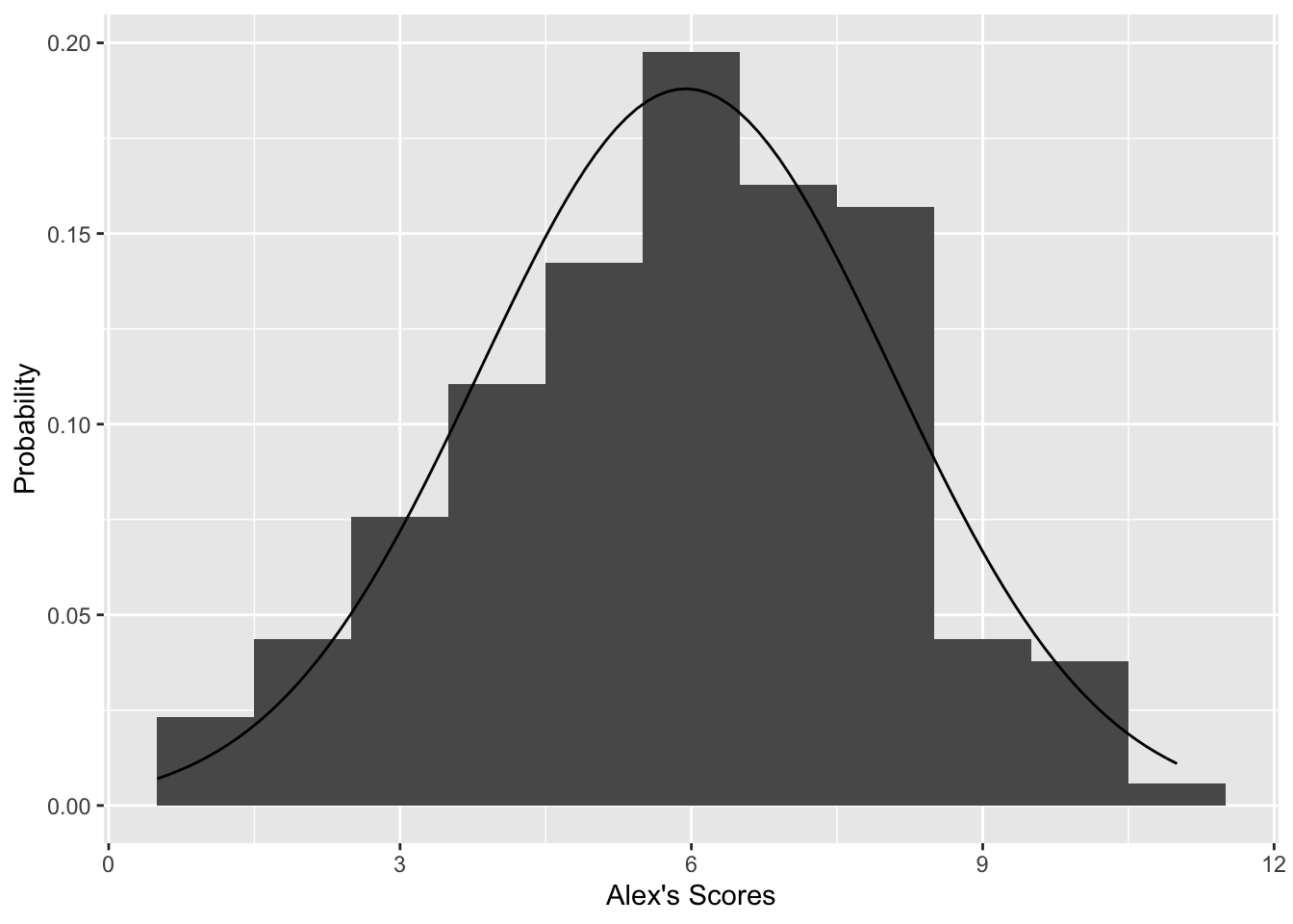
randomUnif <- runif(length(na.omit(allScores$Alex)), -0.5, 0.5)
qqData <- na.omit(allScores$Alex) + randomUnif
qqnorm(qqData)
qqline(qqData)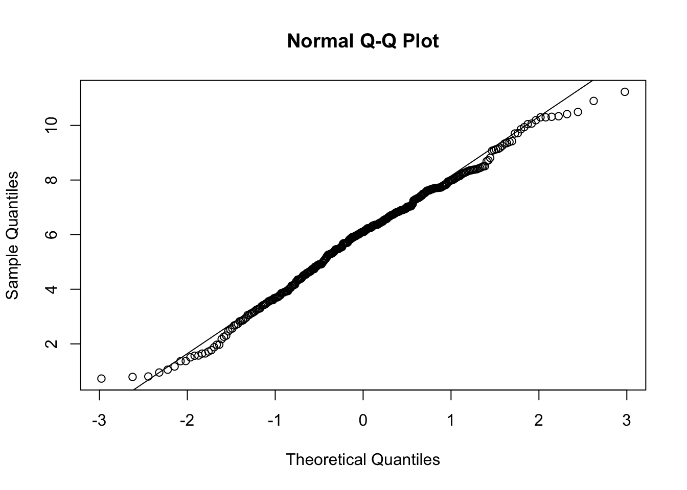
suppressWarnings(ks.test(na.omit(allScores$Alex), "pnorm",
        mean(allScores$Alex, na.rm = TRUE),
        sd(allScores$Alex, na.rm = TRUE)))
One-sample Kolmogorov-Smirnov test
data: na.omit(allScores$Alex)
D = 0.11549, p-value = 0.0002069
alternative hypothesis: two-sidedSo maybe the tails are a bit light for a normal distribution. I doubt anyone will notice the difference during trivia night.
Thing 1: Human Alex’s average round score
Now we look at how roboAlex uses each piece of information it has available. The first thing measures how good human Alex is at Hail Science trivia in general.
library(ggplot2)
meanAlex <- mean(allScores$Alex, na.rm = TRUE)
meanAlex
[1] 5.942326This quantity represents the base score that roboAlex predicts human Alex will score on a given round, without any additional information.
Thing 2: Did human Alex joker this round?
Human Alex picks rounds based on the theme and creator of each round. roboAlex does not know about those things. Naive little roboAlex trusts that human Alex knows what he is doing. roboAlex assigns Alex’s mean score on joker rounds as the base score for his joker round. When I compared roboAlex’s predicted score on joker rounds to real Alex’s actual scores, they tended to be lower, so this adjustment helps.
There is still a flaw here. By using human Alex’s mean joker score as the base score and also taking into account everyone else’s scores, I’m double-counting some of the information about creator and theme. That gives roboAlex a bit of an extra advantage on joker rounds. Luckily, roboAlex 1.0 also tends to underperform on non-joker rounds, so those flaws come reasonably close to evening out.
get_average_joker_round("Alex")[1] 7.252909That score represents the base score that roboAlex predicts Alex will score on a joker round, without any additional information.
Thing 3: How well did everyone else do on this round?
Knowing how well everyone else did on a round makes roboAlex more realistic in two ways. First, if a round is difficult, players tend to score lower, and roboAlex can adjust his score down accordingly. Second, some players’ scores tend to be more predictive of Alex’s score than others.
For example, I would hope to see roboAlex doing better on rounds where Dad and Ichigo also performed well. Likewise, if Mom does really well, it is more likely to be a round that human Alex is not good at. We represent those relationships, plus the shared influence of overall round difficulty, in a covariance matrix.
| Player | Zach | Megan | Ichigo | Jenny | Mom | Dad | Chris | Alex | Jeff | Drew |
|---|---|---|---|---|---|---|---|---|---|---|
| Drew | 0.17 | 0.13 | 0.17 | 0.06 | 0.38 | 0.26 | 0.33 | 0.25 | 0.22 | 0.97 |
| Jeff | 0.00 | 0.10 | 0.05 | 0.04 | 0.04 | 0.33 | 0.05 | 0.24 | 0.64 | 0.22 |
| Alex | 0.28 | 0.39 | 0.46 | 0.22 | 0.15 | 0.57 | 0.44 | 0.93 | 0.24 | 0.25 |
| Chris | 0.24 | 0.27 | 0.23 | 0.15 | 0.24 | 0.27 | 0.98 | 0.44 | 0.05 | 0.33 |
| Dad | 0.29 | 0.36 | 0.21 | 0.27 | 0.19 | 0.96 | 0.27 | 0.57 | 0.33 | 0.26 |
| Mom | 0.16 | 0.45 | 0.21 | 0.38 | 0.98 | 0.19 | 0.24 | 0.15 | 0.04 | 0.38 |
| Jenny | 0.34 | 0.55 | 0.19 | 1.00 | 0.38 | 0.27 | 0.15 | 0.22 | 0.04 | 0.06 |
| Ichigo | 0.17 | 0.33 | 0.88 | 0.19 | 0.21 | 0.21 | 0.23 | 0.46 | 0.05 | 0.17 |
| Megan | 0.44 | 0.99 | 0.33 | 0.55 | 0.45 | 0.36 | 0.27 | 0.39 | 0.10 | 0.13 |
| Zach | 0.60 | 0.44 | 0.17 | 0.34 | 0.16 | 0.29 | 0.24 | 0.28 | 0.00 | 0.17 |
Darker green means stronger covariance. The preserved values match the original post’s covariance display.
covTable <- get_player_covariance_scores()Putting it all together - Prediction
The mean values and covariances are the only variables we need to simulate what is called a conditional multivariate normal distribution. All we need now are the proper equations.
It is important to note that just because each player’s scores follows an approximate normal distribution does not mean the joint distribution will follow a multivariate normal. I’m assuming that here without proof, because the approximation seems to work well enough in this simple setting.
Penn State has a good explanation of the math behind the conditional multivariate normal, but this is the equation the post uses:
E(Y|X = x) = μY + ΣYX ΣX-1 (x - μX)E(Y|X = x) is the prediction: how well roboAlex is expected to score given that everyone else scored x.
μY is how well human Alex scores on an average round, or on a joker round if this is a joker.
ΣYX is the row of the covariance matrix corresponding to Alex, without the Alex/Alex entry.
ΣX-1 is the precision matrix: the covariance matrix with Alex’s row and column removed, then inverted.
This is where most of the “don’t double-count correlated players” magic happens.
(x - μX) is everyone else’s performance on this round relative to their average score. Once multiplied through,
the terms tell us how much each observed player performance should push Alex’s estimate up or down.
This still underestimates Alex a little because the round creator usually does not have a score entered on their own round. So if Ichigo created the round, her normally useful contribution to the estimate is missing. The post notes a few ways to fix that later.
Putting it all together - Simulation
The best estimate of how well real Alex will perform is given by the prediction above. But if roboAlex always predicts the expected score, it will never have a truly great or truly terrible night. To make roboAlex feel like a real trivia player, the model also keeps the right amount of variance:
Var(Y|X = x) = ΣY - ΣYX ΣX-1 ΣXYIn English, the model starts with Alex’s natural score variability and removes some of it because the other players’ scores tell us something about what kind of round this was.
All that is left is to draw random samples from the resulting normal distribution. The rest of the post tries a few scenarios and compares the simulated distributions to Alex’s historical one.
Sigma_XY <- covTable[c(1:7, 9, 10), 8]
Sigma_YX <- covTable[c(1:7, 9, 10), 8]
Sigma_X  <- covTable[c(1:7, 9, 10), c(1:7, 9, 10)]
Sigma_Y  <- covTable[8,8]

meanPlayerScores <- c(mean(allScores$Zach, na.rm = TRUE),
                      mean(allScores$Megan, na.rm = TRUE),
                      mean(allScores$Ichigo, na.rm = TRUE),
                      mean(allScores$Jenny, na.rm = TRUE),
                      mean(allScores$Mom, na.rm = TRUE),
                      mean(allScores$Dad, na.rm = TRUE),
                      mean(allScores$Chris, na.rm = TRUE),
                      mean(allScores$Jeff, na.rm = TRUE),
                      mean(allScores$Drew, na.rm = TRUE))
set.seed(6)
roboAlexMean <- meanAlex + Sigma_YX %*% solve(Sigma_X) %*% c(0, 0, 0, 0, 0, 0, 0, 0, 0)
roboAlexVariance <- Sigma_Y
predictions <- data.frame("preds" = rnorm(388, roboAlexMean, sqrt(roboAlexVariance)))
hist(predictions$preds, col = rgb(1,0,0,0.5), xlim = c(0,12), prob = TRUE,
main = "Histogram of simulated (red) vs actual (blue) round scores", xlab = "Score")
hist(allScores$Alex, col = rgb(0,0,1,0.5), add = TRUE, prob = TRUE)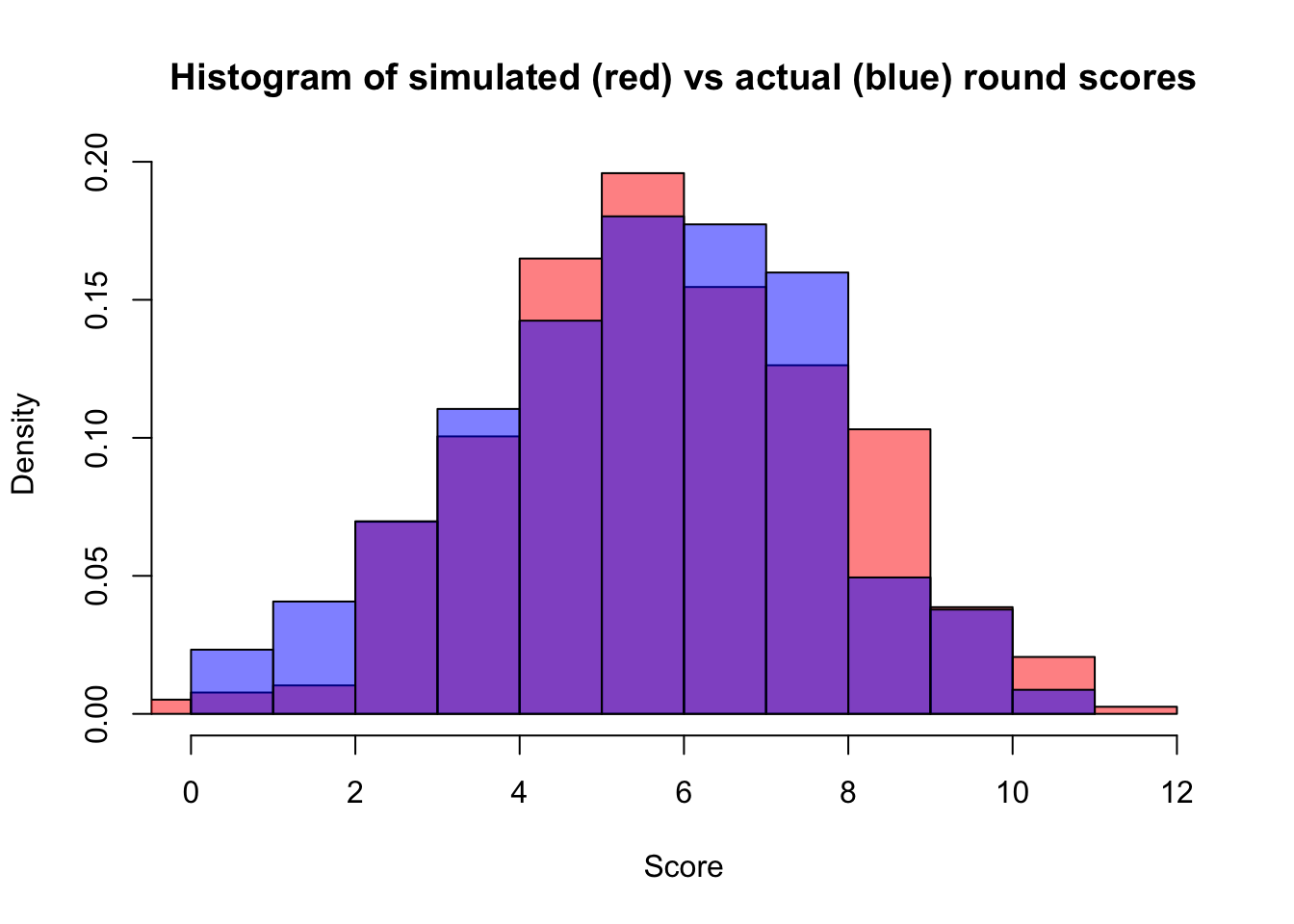
Not bad. Now let’s tell roboAlex that everyone did exactly as well as average and see how that changes the estimate.
set.seed(6)
roboAlexMean     <- meanAlex + Sigma_YX %*% solve(Sigma_X) %*% c(0, 0, 0, 0, 0, 0, 0, 0, 0)
roboAlexVariance <- Sigma_Y - Sigma_YX %*% solve(Sigma_X) %*% Sigma_XY
predictions      <- data.frame("preds" = rnorm(388, roboAlexMean, sqrt(roboAlexVariance)))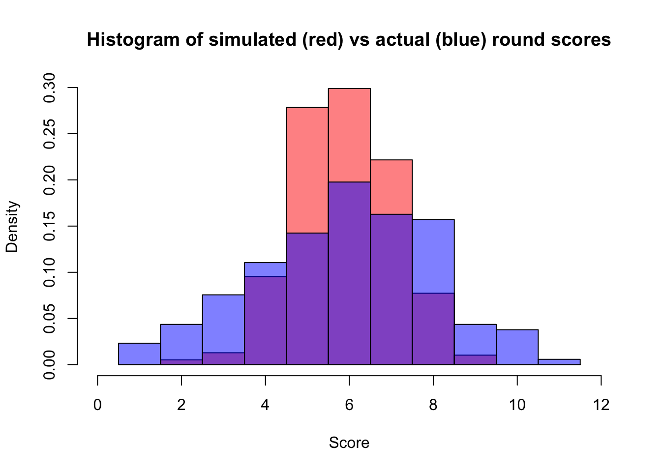
Seems reasonable: if everyone got a middling score, we are a lot more confident that human Alex would have as well. What about one of those rounds about animated TV that Jenny, Zach, and Megan always do well on but no one else does?
set.seed(6)
sampleScores      <- c(8, 8, 5, 9, 4, 3, 4, 3, 3)
roboAlexMean      <- meanAlex + Sigma_YX %*% solve(Sigma_X) %*% (sampleScores - meanPlayerScores)
roboAlexVariance  <- Sigma_Y - Sigma_YX %*% solve(Sigma_X) %*% Sigma_XY
predictions       <- data.frame("preds" = rnorm(388, roboAlexMean, sqrt(roboAlexVariance)))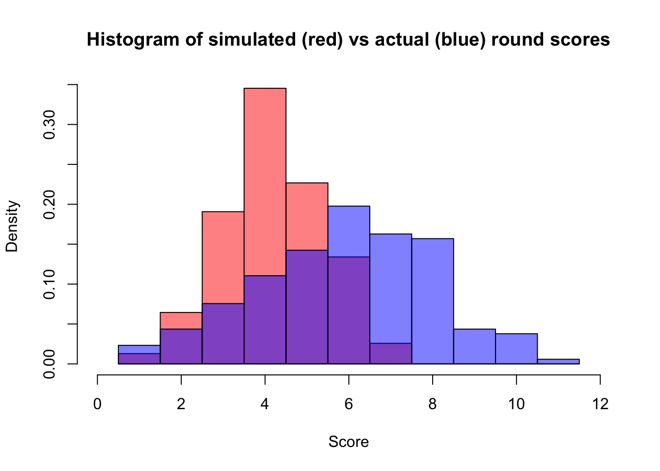
Yep. What about an easy round where everyone does well? Again, the original post treats this as a quick plausibility check rather than a full historical validation.
set.seed(6)
sampleScores      <- c(8, 8, 9, 9, 9, 10, 8, 9, 8)
roboAlexMean      <- meanAlex + Sigma_YX %*% solve(Sigma_X) %*% (sampleScores - meanPlayerScores)
roboAlexVariance  <- Sigma_Y - Sigma_YX %*% solve(Sigma_X) %*% Sigma_XY
predictions       <- data.frame("preds" = rnorm(388, roboAlexMean, sqrt(roboAlexVariance)))
predictions$preds[which(predictions$preds > 10)] = 10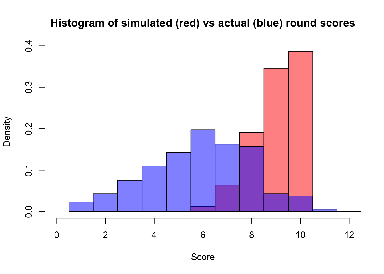
Dad scoring a 10 and Ichigo getting a 9 both help a lot, and roboAlex ends up with close to an even chance of either score. The predicted values above 10 were truncated, assuming there were no bonus questions. The behavior felt plausible enough that roboAlex started to look like a real stand-in player.
That’s all for now.
Coming in version 1.1 / 1.2
- Fix the overestimation on joker rounds by comparing estimated joker scores with historical joker-round performance.
- Fix the general underestimation by accounting for round creator more explicitly, possibly with creator-specific covariance matrices.
- Collect historical data on scenarios like easy rounds or certain themes to check calibration more directly.
- Try using htmlwidgets to make an interactive roboAlex predictor using sample sets of scores.
- Normalize round scores, since the non-normality may partly come from rounds being out of different totals.
- Later on, possibly adjust for round theme directly and remove the separate joker-round score shortcut.